chapter 6 b
CHAPTER6 (Better discussion from Foley)
Local Illumination and Shading Models
The theory behind shading objects is based on their position, surface properties, the lights used in a scene, and the position of the observer. Each model addresses either some or all of these issues.
An illumination model is used to determine the surface color of an object at a given pixel.
A shading model defines when an illumination model is applied and what parameters it needs to determine the color of an object.
Many of the illumination models currently used were developed in the early 60's. Graphics researchers at that time approximated the rules for optics and thermal radiation in order to simplify the models which resulted in more efficient color calculation. Even though these models are often kludges, using clever heuristics, they do a surprisingly realistic job.
Simple Illumination Model
The simplest illumination model contains no light source but merely assumes that each object in a scene radiates a color based on the properties of the object.
A scene rendered with this simple model looks pretty unrealistic because each object is non-relective and self-luminous. Objects appear to have a matte, flat, and monochromatic look.
The simple illumination model is expressed as
I = ki, where I is the color intensity of an object with color property ki.
Color calculation in such a model is trivial since all points on the surface have color = ki.
In openGL this model is captured through "emissive light" from the object. Since this is a surface property it is defined through an openGL material property command:
void glMaterial[if][v](GLenum face, GLenum pname, TYPE
            [*]param);
where a possible setup might be:
GLfloat mat_emission[] = { 0.3,0.2,0.3,1.0}; //emissive
            color
glEnable(GL_LIGHTING);
glEnable(GL_DEPTH_TEST);
...........................
glMaterialfv(GL_FRONT,GL_EMISSION,mat_emmission);
glutSolidCube(1.0);
Ambient Light Illumination Model
The ambient illumination model expands on the simple model by assuming a diffuse nondirectional light source. Now instead of self-luminosity, the color of an object depends on the light radiated by all objects in the scene. It is assumed that this radiated light affects all objects equally. The radiated enviromental light is referred to as ambient light.
The ambient illumination model is expressed as
I = Ia*ka, where I is the color intensity of the object.
- Ia is the ambient color intensity which is equal for all objects
- ka is the ambient reflection coefficient (arc). Arc is an ambient surface property which is unique for each object and whose value is in the interval [0,1]. The arc does nor correspond to any real physical properties of objects but was developed through empirical studies - it produces fairly realistic looking objects.
Although ambient lit objects are more realistic-looking than in the self-luminous case they are still only uniformly lit across their surfaces
We have direct experience with this model since it is the default illumination model used in openGL. Defining a light with:
void glLight[if][v](GLenum light, GLenum pname, TYPE
            [*]parm);
and possible setup of model:
GLfloat light_pos[] = {1.0,1.0,1.0,1.0}; //light
            position
GLfloat light_ambient[] = {0.5,0.0,0.0,1.0}; //ambient
            light intensity
GLfloat mat_ambient[] = { 0.2,0.2,0.2,1.0}; /*ambient
            color ~ ka, no direct correlation in openGL.*/
glLightfv(GL_LIGHT0,GL_POSITION,light_pos); //up to 8
            lights may be specified [0..7]
glLightfv(GL_LIGHT0,GL_AMBIENT,light_ambient);
glEnable(GL_LIGHTING);
glEnable(GL_LIGHT0);
glEnable(GL_DEPTH_TEST);
...............................
glMaterialfv(GL_FRONT,GL_AMBIENT,mat_ambient);
glutSolidCube(1.0);
Diffuse Reflection Illumination Model
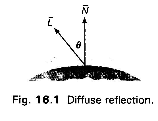
The diffuse reflection model assumes a positional light source that radiates light uniformly in all directions. In such a model, the color of a point on the surface of an object should depend on its orientation to and distance from the light source.
Lambertian reflection attempts to model the diffuse reflection of dull matte surfaces. Such surfaces reflect light equally in all directions. Thus the brightness of such a surface depends only on the angle theta between two vectors given by
- L = direction from a point on the surface to the light source
- N = normal at the point on the surface. See figure 16.1.
Why is this dependency true?
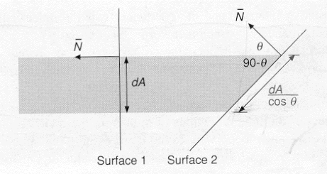
The area intercepted by a light beam is proportional to cos (theta): dA/cos (theta). This is true for all surfaces no matter their surface properties.
Assume the point light source radiates a light beam with an infinitesimally small cross sectional area, dA. Now visualize this beam intercepting the surface of an object at the normal N.
a). In the case where N = L the beam intersects an area on the surface which is equal to dA ?=> Since N = L then theta = 0 and cos(0) = 1 thus the area intercepted by the beam is dA/(cos theta) = dA/1 = dA. Surface 1 above.
b). In the case where N != L, the angle theta is in the interval (0,90) ?=> the 0 case was handled in a)., theta must be less than 90 degrees otherwise L is perpendicular to N and the surface is a back face => not lit. The cos theta for theta in the interval (0,90) is 0 < cos theta < 1. Thus the area intercepted by the beam is dA/cos theta > dA. This is exactly what we would expect: as the angle between the light source and the normal increases the intercepted area also increases.
Lambertian surfaces adher to Lambert's law which states that the amount of light reflected from the intercepted area dA to the viewer is directly proportional to the cosine of the angle between the normal, N, and the direction to the viewer, D. Again this is what we would expect. As the angle between the normal and the direction to the viewer increases less light is reflected back to the observer.
The amount of surface area seen by an observer is inversely proportional to the cosine of the angle between the normal and the direction to the observer. This makes sense because as the angle increases between N and D, more surface area is exposed to the viewer.
Thus, combining Lambert's law defining brightness of reflected light (directly proportional to cos theta) with amount of surface area seen (inversely proportional to cos theta) causes the two factors to cancel each other out.
Q.E.D. The brightness of a Lambertian surface depends only on the angle theta between N and L.
The diffuse illumination equation is
I = Id*kd*(cos theta) where
- Id is the intensity of the point light source.
- Kd is the object's material property referred to as the diffuse-reflection coefficient (drc) and varies over the interval [0,1]. Drc has been determined through empirical studies.
The equation can be restated as :
I = Id*kd*(N.L) where . is used to denote dot product and N, L must be normalized.
In what coordinate system must the illumination equation be evaluated?
If the equation is evaluated after projection then the angle theta may be modified resulting in incorrect color determination. Therefore evaluation must be performed in the world-coordinate space.
If the light source is changed to a directional light source (a light source which is very far from all objects) then its vector makes the same angle with all surfaces sharing the same surface normal and L is a constant for the light.
Diffuse illumination results in very harshly lit objects. For this reason, both a diffuse and an ambient component are combined as in
I = Ia*ka + Id*kd*(N.L).
Refer to Nate Robbins Lighting Tutors (demoed in class) to see how modifying ka and kd in the two models (diffuse vs ambient-diffuse) affects the look of objects.
The diffuse and ambient-diffuse models are supported in openGL (simply remove the ambient calls to get straight diffuse):
Note that it is possible to set the ambient and diffuse material properties to the same color using
glMaterialfv(GL_FRONT,GL_AMBIENT_AND_DIFFUSE


            ,mat_ambient);
GLfloat light_pos[] = {1.0,1.0,1.0,0.0}; //light
            position - this is a directional light
GLfloat light_ambient[] = {0.5,0.0,0.0,1.0}; //ambient
            light intensity
GLfloat light_diffuse[] ={1.0,1.0,1.0,1.0}; //diffuse
            light intensity
GLfloat mat_ambient[] = { 0.2,0.2,0.2,1.0}; //ambient
            color
GLfloat mat_diffuse[] = { 0.5,0.2,0.0,1.0}; /*diffuse
            color~kd, no direct correlation in openGL*/
/*using a directional light where L is constant, for a
            point (positional) light source set
w coordinate to a non-zero value as inGLfloat light_pos[] = {0.0,0.0,1.0,1.0};*/
glLightfv(GL_LIGHT0,GL_POSITION,light_pos);
glLightfv(GL_LIGHT0,GL_AMBIENT,light_ambient);
glLightfv((GL_LIGHT0,GL_DIFFUSE,light_diffuse);
//do the enable stuff for lights
...............................
glMaterialfv(GL_FRONT,GL_AMBIENT,mat_ambient);
glMaterialfv(GL_FRONT,GL_DIFFUSE,mat_diffuse);
glutSolidCube(1.0);
Light Source Attenuation
When two parallel surfaces, with exactly the same material properties, overlap it is not possible to distinguish this overlap (no matter the differences in their distance from the light source) with the models discussed so far. To do so requires adding an attenuation factor, fatt, to the light source giving the new illumination model as:
I = fatt*(Ia*ka + Id*kd)
Note that adding an attenuation factor for a directional light source makes no sense. The attenuation factor causes the intensity of the light source to decrease as the distance from the light increases. The attenuation factor can be defined in several ways:
- fatt = 1/(d*d) where d is the distance from the light to the surface. This is not the best function as objects very far from the light don't show much variation while those close to the source vary widely.
- fatt = min(1/(c1+c2*d+c3*d*d), 1) where c1,c2,c3 are user defined. The function is clamped to 1 as a maximum and c1 keeps the denominator from becoming too small when the light is close to the object.
openGL supports the fatt as defined in ii). The default values for the constants are c1 =1.0, c2 = 0.0, and c3 = 0.0. Such a setting gives a constant attenuation. You can change the defaults using
glLightf(GL_LIGHT0, GL_CONSTANT_ATTENUATION,2.0);
            //sets c1
glLightf(GL_LIGHT0, GL_LINEAR_ATTENUATION,1.0); //sets
            c2
glLightf(GL_LIGHT0, GL_QUADRATIC_ATTENUATION,0.5);
            //sets c31
Note that all components of the light are attenuated (ambient, diffuse, and specular). Attenuation is set to 1 in openGL when using a directional light source.
Colored Lights and Surfaces for the Ambient-Diffuse Model
As we would expect, the color of a surface is a combination of its surface color properties and the color of any lights in the scene. If we just look at the red intensity of an object it would be determined as:
Ir = fatt*(Ia*ka*Oa + Id*kd*Od*(N.L)).
This is the model used in openGL when combining colored positional lights and colored surfaces (with the omission of ka and kd).
Note that the values provided for lights as in:
GLfloat light_ambient[] = {0.5,1.0,0.0,1.0};
signify a percentage of full color intensity.
The values provided for materials as in :
GLfloat mat_ambient[] = { 0.5,0.5,0.0,0.0};
signify the reflected proportions of colors. In the example, the surface reflects half the red/green light and none of the blue. The total reflected red is .5*.5 or .25 and the total reflected green is 1.0*.5 or .5.
Atmospheric Attenuation
In order to approximate an atmosphere separating an object from the viewer, depth cues are used in many systems. In openGL this is done using the fog atmospheric condition which works according to the model given in the text/Redbook. Read on your own.
Specular Reflection
Specular reflection occurs when a light source strikes a shiny object creating a highlight. The highlight color is affected by the color of the incident light from the light source. The highlight moves as the observer's position moves because shiny surfaces reflect light unequally in different directions.
Diagram : reconstruct the vectors used for the diffuse
reflection illumination model : N, the surface normal, L, the
vector to the light source, V the vector to the viewpoint. N and
L form an angle of theta. Reflect L around N to produce the
reflection vector R. R and N form an angle of theta. R and V
form an angle of alpha. 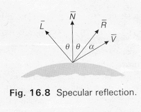
If our object is a perfect reflector (a mirror) then light is reflected only in the direction of R. The observer would see the specularly reflected light only if they were positioned at R or when alpha = 0.
The Phong Illumination Model for Specular Reflection
Phong's model is used to handle non-perfect reflectors. The assumption made in this model is that maximum specular reflection occurs when alpha = 0 (angle between R and V) and then falls off rapidly as alpha increases. The rapid falloff is captured via:
cosn(alpha), n is a material property called the specular-reflection exponent. Values for n range from 1 to several hundred. Low values give soft gentle highlights while high values give sharp focused highlights.
The Phong illumination model is stated as :
I = fatt*(Ia*ka*Oa + Id[kd*Od*(N.L)] + Is*ks*Os(R.V)n) here ks is the specular reflection coefficient of the object and n is the shininess.
Note that this model captures the ambient, diffuse and specular properties of lights and surfaces. Here, Od, and Os capture the diffuse, and specular material properties (as in openGL). The ka, kd, and ks coefficients are NOT supported in openGL. The specular reflection coefficient (n) is supported in openGL and must be in the interval [0,128].
An example to just set up the specular stuff is:
GLfloat light_pos[] = {1.0,1.0,1.0,1.0}; //light
              position
GLfloat light_specular[] ={1.0,1.0,1.0,1.0}; //white
              light
GLfloat mat_specular[] = { 1.0,1.0,1.0,1.0};
GLfloat shininess[] ={50.0};
//specular reflection coefficient.
glLightfv(GL_LIGHT0,GL_POSITION,light_pos);
glLightfv(GL_LIGHT0,GL_SPECULAR ,light_specular);
....................
glMaterialfv(GL_FRONT,GL_SPECULAR,mat_specular);
glMaterialfv(GL_FRONT,GL_SHININESS,shininess);
Multiple Light Sources and Odds/Ends
If multiple light sources are used then the attenuation/diffuse and specular components of each light is summed and then added to the single ambient component to get the final color intensity, I. To ensure against overflow (color values > 1.0) the intensity of I is clampled to 1.0.
It should be clear that a single light source (with all the bells and whistles) adds considerable overhead to the color calculation of a fragment. Multiple lights increase the problem, but can be used for nice effects.
openGL supports directional, positional and spot lights (read on your own).
openGL allows you to specify a stationary light, a light that moves independently of objects in the scene, and one that moves with the observer.
- Stationary Light : any modifications to the ModelView matrix also affect the position of the light source. To keep the light stationary, set its position only after performing all model view transformations.
- Independent Light : apply model view transformations to the light position command. If you want these to be independent of the transformations applied to the object then isolate the transformations in a push/pop matrix block. Any transformations applied to the object also affect the light.
- Moves with the Viewpoint : set the light position before setting any viewing transformations. Since the initial viewpoint is at 0,0,0, the light position might be initialized equivalently. Application of viewing transformations will now move the light along with the observer at a distance of 0,0,0. Of course, specifying the light position at some distance from the viewpoint will keep this distance constant when applying viewing transformations.
We have discussed viewing transformations. The modelview matrix mode composes all transformations applied to objects (models) and the observers position (viewpoint). The viewpoint can be moved via the following openGL command :
void gluLookAt(GLdouble ex, GLdouble ey, GLdouble ez,
              GLdouble cx, GLdouble cy, GLdouble cz, GLdouble upx,
              GLdouble upy, GLdouble upz);
- The observers position is captured by ex,ey,ez
- the observers line of sight (a point in the scene) is defined by cx,cy,cz
- upx,upy,upz specify which direction is up. Typically upy = 1.0.
Lighting Model Selection : openGL allows the programmer to specify 4 components of the lighting model used in a scene.
- 1. Global Ambient Ilumination for the scene :
GLfloat lmodel_ambient[] = {0.2,0.2,0.2,1.0};
                    //default value
glLightModelfv(GL_LIGHT_MODEL_AMBIENT, lmodel_ambient); - 2. Whether the viewer is local to the scene or
considered to be at an infinite distance from the scene
(default). When the viewpoint is local to the scene then
specular highlight intensity depends on the vertex normal,
light vector, and viewer vector. Defining a local
viewpoint gives more realistic results but incurs the
overhead of normal/vector determination.
glLightModeli(GL_LIGHT_MODEL_LOCAL_VIEWER,GL_TRUE); - 3. Whether to use one-sided or two-sided lighting (for
cut-away display of objects for example):
glLightModeli(GL_LIGHT_MODEL_TWO_SIDE, GL_TRUE); - 4. To separate specular color from ambient (for more realistic texture mapping lighting results - not supported in version 1.2 of openGL...checking on later versions).
Polygon Shading Models
Flat Shading
The simplest shading model is flat shading. In this model, polygonal boundaries can be seen and the object has a faceted appearance. The approach applies the illumination model once to compute a single color intensity that is then used to color the entire surface of a polygon.
This approach only makes sense if
- the light source is at infinity (N'L is constant across the face of the polygon)
- the observer is at infinity (N'V is constant)
- the polygon is not an approximation of a curved surface.
If either 1). or 2). is not true then constant shading can still be carried out by computing the normal, light and viewer vectors once. Typically the center of the polygon or the first vextex of the polygon is used for the vector determination.
Interpolated Shading
As an alternative to flat shading, an illumination model might carry out the illumination calculation for each pixel that intersects the surface of a polygon. For a large complex scene with many polygons such an algorithm would be prohibitively expensive.
Algorithms that approximate the above brute force illumination calculation use interpolated shading. Gouraud smooth shading is probably the best known and most general of the interpolated shading algorithms. Phong smooth shading is a more costly interpolated algorithm but one which produces better results. Both are discussed later.
Shading of polygon meshes that approximate a curved surface must address some interesting problems.
- Adjacent polygons within the mesh might exhibit very different orientations. Vector calculations for the lighting model will produce very different color intensities for neighboring polygons in this instance. The mesh will have a faceted appearance whether constant shading or interpolated shading is used.
- Increasing the number of polygons in the mesh will only accentuate the problem: known as the Mach band effect. The Mach band effect has to do with the way receptors in the eye react to light intensity changes. The easiest way to understand the Mach band effect is to look at the perceived intensity change where two walls of a room intersect. There appears to be a darker band (near the intersection) along the wall with a lower light intensity. This effect is only a perceived one and not an actual intensity change. Mach banding can make a fine grained polygon mesh look pretty awful.
Smooth shading of polygonal meshes attempts to address the faceting problem and the Mach band effect by using color information from adjacent polygons within the mesh. How this is done is discussed in the following sections.
Gouraud Smooth Shading
Gouraud shading is a color interpolation algorithm that eliminates most but not all Mach banding problems (still evident when a very rapid intensity change occurs).
What are the basics of color interpolation?
- Assume the polygon to be shaded is a triangle and that the three vertex normals are available.
- A selected illumination model can then be used to determine the color intensity for the three vertices: I1, I2, I3.
- The linear color interpolation occurs during scan line conversion and is a very efficient incremental algorithm.
- Assume that vertex1 with intensity I1 intersects scanline y1, vertex2 with I2 intersects scanline y2, and vertex3 with I3 intersects scanline y3.
- The algorithm must be able to determine the color intensity across all scanlines that intersect the triangle.
- Assume an arbitrary scanline ys, intersects the polygon.
- Let the intensity at the left intersection of the polygon and the scanline = Ia, and at the right edge = Ib. Ia and Ib are calculated as follows :
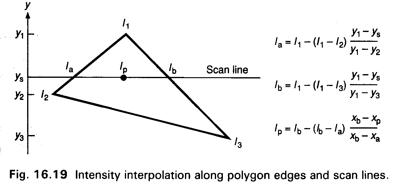
Ia = I1 - (I1-I2)*(y1-ys)/(y1-y2)
Ib = I1 - (I1-I3)*(y1-ys)/(y1-y3)
To find the intensity, Ip of a point along the edge defined by the left and right intersections of the scanline and the polygon use :
Ip = Ib - (Ib - Ia)*(xb-xp)/(xb-xa)
Gouraud shading requires that
- The normal at each vertex of the polygon is known. If the vertex normals are not directly available they may be calculated by averaging the surface normals of all polygons incident on the vertex.
- Apply an illumination model using the vertex normals to calculate a vertex color intensity.
- Apply linear color interpolation across all scanlines intersected by the polygon. The linear interpolation is made more efficient by using a difference equation (as in the scan conversion algorithm)=> an incremental change in y over intersecting scanlines, and an incremental change in x across the scanline.
Phong Smooth Shading
Phong's model also uses linear interpolation but here the normal vector is the interpolated value and not color intensities. The model requires that vertex normals are available or determined through averaging. The linear interpolation of normal vectors proceeds as in Gouraud shading and the interpolation is applied to the three components of the vector.
Previously we discussed the fact that illumination models must be applied in the world coordinate system because perspective transformation can modify the angles between N, L, V, and R, producing incorrect lighting results.
- In Gouraud's algorithm color intensity at a vertex is determined by applying the illumination calculation in world coordinate space and all proceeds correctly.
- In Phong's algorithm the color calculation is performed
during rasterization (in screen coordinate space) which
complicates matters significantly.
- The normal at each pixel along the scanline must be normalized and mapped back into world coordinate space where the illumination model is then applied. This process is very costly and only makes sense if the rendered image is to faithfully capture realistic specular reflections.
What does the Phong model give you that Gouraud's does not?
Refer to figure 16.21 of text. 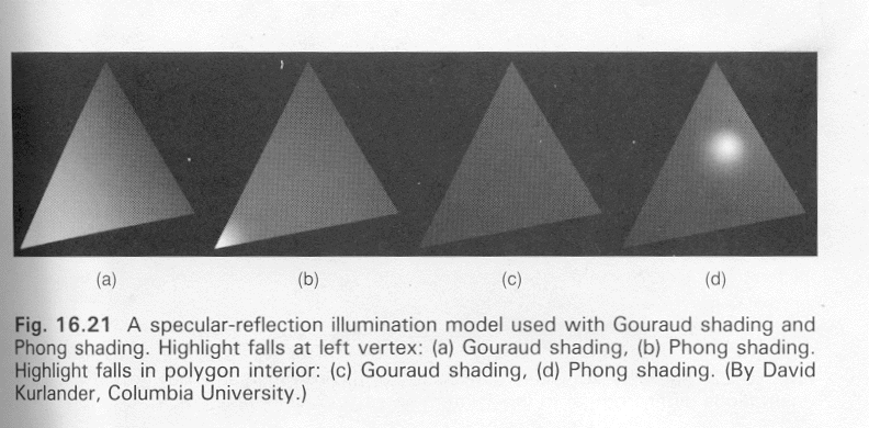
a). If a highlight falls on a vertex : G's model will interpolate the highlighted vertex with the non-highlighted vertices. This does not produce a highlight but a lighter intensity that gradually darkens across the face of the polygon.
b). P's model accurately reproduces the vertex highlight.
c). If the highlight falls in the interior of the polygon : G's model interpolates only non-highlighted vertices so no highlight is produced.
d). P's model captures the interior highlight.
e). Mach banding : G's model alleviates many mach banding effects while P removes all effects.
Problems with Interpolated Shading
- The polygonal silhouette edges of the object are still visible.
- Perspective distortion causes foreshortening of edges along which the interpolation occurs.
- Orientation dependence can cause the same point on the surface to have different intensities as the surface rotates. This happens because the intersecting scanline with the polygon will have different lengths dependent on the geometry of the polygon. Because the interpolation occurs across the intersecting scanline the interpolated values may be quite different for the same point.
- If two adjacent polygons do not share a vertex along a common edge then color discontinuity can arise.
- Unrepresentative vertex normals.
Adding Surface Detail to Objects
- Simply add some additional surface polygons to a base polygon (i.e. polygons representing doors, windows, or lettering) => Surface Detail Polygons.
- Texture Mapping
- A technique to map an image onto a surface to approximate detail. The process was developed by Catmull in 1974 and refined by Blinn and Newell in 1976. Although maps may be 1-D, 2-D, or 3-D this discussion deals only with 2-D maps.
Texture Mapping (OpenGL
Redbook Texture discussion)
The image to be applied is called a texture map with individual components of the map referred to as texels. The map resides in a 2-D texture coordinate space, with coordinates specified by (s, t).
The texture mapping algorithm is a two step process that
occurs during rasterization. 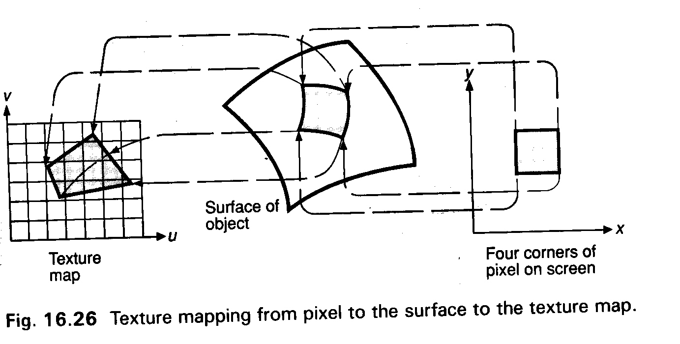
- The four corners of a screen pixel are mapped onto the surface of the object that the pixel intersects.
- The surface may be curved.
- The four corners of the surface pixel are then mapped onto the texture.
- The texture pixel is defined by four corners in (s, t) space and is a quadrilateral.
- This quadrilateral will only be an approximation of the surface pixel if the surface is curved.
- Each texel color is weighted based on the proportion of the area of the quadrilateral it occupies.
- The color intensity of the screen pixel is then determined by summing all the weighted texel colors.
If the (s, t) coordinates fall outside of the map, then one can think of the map as being replicated. The mapping proceeds as described above.
If the surface to be mapped is a polygon then it is advantageous to assign texture coordinates directly to the polygon vertices. Linear interpolation of the texture coordinates can be applied during scanline conversion.
Again, due to orientation-dependence, interpolating can cause texture distortion due to the foreshortening that occurs with perspective transformation.
It should be obvious that texturing is an expensive process
- the two step mapping process
- application of a filter (perhaps more complex than the simple box filter described above)
- summing of texels
=> hardware support is highly desirable.
Texture Mapping in openGL
A very large and complicated topic area of openGL. The following discussion is not all inclusive, deals only with 2-D issues.
Texture mapping is performed in RGBA mode.
The steps to get a texture going are :
- Create a texture object and specify a texture for the
object.
- A texture can be loaded from a file or produced by the application program. If you are interested in program created textures then refer to the Texture Chapter in the openGL book for several examples. The following deals only with .rgb texture files. Examples for reading and using different image files can be found in the GamingTutors/GamingTutorsPCWinandGlut/Textures folder.
Example
//loading the texture filechar* filename;RGBImageRec *image = NULL;image = rgbImageLoad(filename);//create the texture objectglPixelStorei(GL_UNPACK_ALIGNMENT,1);GLuint whichTexture; //texture IDglGenTextures(1, &whichTexture); /*returns 1 unused texture ID*/glBindTexture(GL_TEXTURE_2D, whichTexture); //create and bind the texture to the ID//specify the textureglTexImage2D(GL_TEXTURE_2D, 0,GL_RGBA, image->sizeX, image->sizeY, 0, GL_RGBA,GL_UNSIGNED_BYTE, image->data);End Example
glPixelStorei
Specifies how to store the pixel data for the image in memory. In this case the data is unpacked and aligned on 2-byte boundaries
glTexImage2D
The first argument should be as specified, the second specifies the number of resolutions required for the map (0), the third describes the internal format of texels in the map [a list of possible values on page 361], width and height of the image are provided next, followed by the size of the texture border, if any. The next two arguments specify the format of the texture image data. The last is a pointer to the texture data. Note that sizeX, sizeY, and data are fields of the RGBImageRec pointer.
- Indicate how the texture is to be applied to each pixel.
- One of four functions can be used to specify how the
final color of a textured fragment is determined.
Typically specified in init.
Replace mode : just use the texture data,
GL_REPLACE.Decal mode : like replace but blends alpha component,
GL_DECAL.Modulate mode : texture is used to scale the fragments color,
GL_MODULATE.Blend mode : blends texture and fragment color,
GL_TEXTURE_ENV_COLOR,

                      GL_BLEND
.
Example
glTexEnvf(GL_TEXTURE_ENV, GL_TEXTURE_ENV_MODE,
                  GL_REPLACE);
End Example
- One of four functions can be used to specify how the
final color of a textured fragment is determined.
Typically specified in init.
- Enable texturing, typically in init, but can be turned
on/off as needed.
glEnable(GL_TEXTURE_2D); - Specify how the texture is to be repeated and filtered
for (s, t) coordinates. The below is a sufficient set.
Example
//how to repeatglTexParameterf(GL_TEXTURE_2D, GL_TEXTURE_WRAP_S, GL_REPEAT); glTexParameterf(GL_TEXTURE_2D, GL_TEXTURE_WRAP_T,GL_REPEAT);/*how to filter: magnify if fragment maps to a small portion of a texel, minify if the fragment maps to a large collection of texels. Third parameter specifies filtering method : nearest => use texel coordinates closest to pixel center, linear => use a weighted sum of 2X2 array of texels that lie nearest to center of pixel.*/glTexParameterf(GL_TEXTURE_2D, GL_TEXTURE_MAG_FILTER, GL_NEAREST); glTexParameterf(GL_TEXTURE_2D, GL_TEXTURE_MIN_FILTER, GL_NEAREST);End Example
Many other options available, listed on page 412.
- Draw the scene supplying texture coordinates and
geometric coordinates. You must specify your own texture
coordinates or allow openGL to compute the coordinates for
you.
Example
/*An example of user defined texture coordinates.
                  Find in the samples/samples1 texture folder.*/
for (i = 0; i < 6; i++) {//draws a cubeglBegin(GL_POLYGON);glNormal3fv(n[i]); glTexCoord2fv(t[i][0]); glVertex3fv(c[i][0]);glNormal3fv(n[i]); glTexCoord2fv(t[i][1]); glVertex3fv(c[i][1]);glNormal3fv(n[i]); glTexCoord2fv(t[i][2]); glVertex3fv(c[i][2]);glNormal3fv(n[i]); glTexCoord2fv(t[i][3]); glVertex3fv(c[i][3]);glEnd();/*An example of openGL computed texture coordinates*/glTexGeni(GL_S, GL_TEXTURE_GEN_MODE, GL_SPHERE_MAP);glTexGeni(GL_T, GL_TEXTURE_GEN_MODE, GL_SPHERE_MAP);glEnable(GL_TEXTURE_GEN_S);glEnable(GL_TEXTURE_GEN_T);auxSolidTorus(1.0,1.0);End Example
Other possibilities for last parameter of TexGen command listed on page 413.
It is possible to change texture parameters and texture generation modes on the fly during execution. All commands stay in effect until disabled or respecified with a new command.
Examples follow.