Curves and Surfaces (from Foley and Van Dam)
Curves and surface modeling are very rich topics in computer graphics. We will touch on three methods to approximate curves and curved surfaces
- polygonal meshes
- parametric curves and surfaces
- quadric surfaces.
Parametric curves are introduced as a preparatory step in understanding parametric surfaces.
OVERVIEW
Polygon Mesh
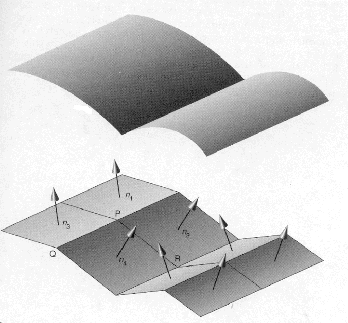
A polygon mesh is a set of connected polygonally bounded planar surfaces. A mesh can be used to represent polygonal objects in a natural manner. A mesh can also be used to approximate a curved surface. Refer to figures below.
Parametric Curve
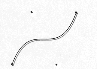
A parametric polynomial curve is used to represent a 3D curve. Points (x, y, z) on the curve are defined by three polynomials, one each for x, y, z. The polynomials are in one parameter, t. Typically, a third degree polynomial is used which produces a cubic curve. This figure depicts a Bezier curve.
Parametric Patches (surfaces)
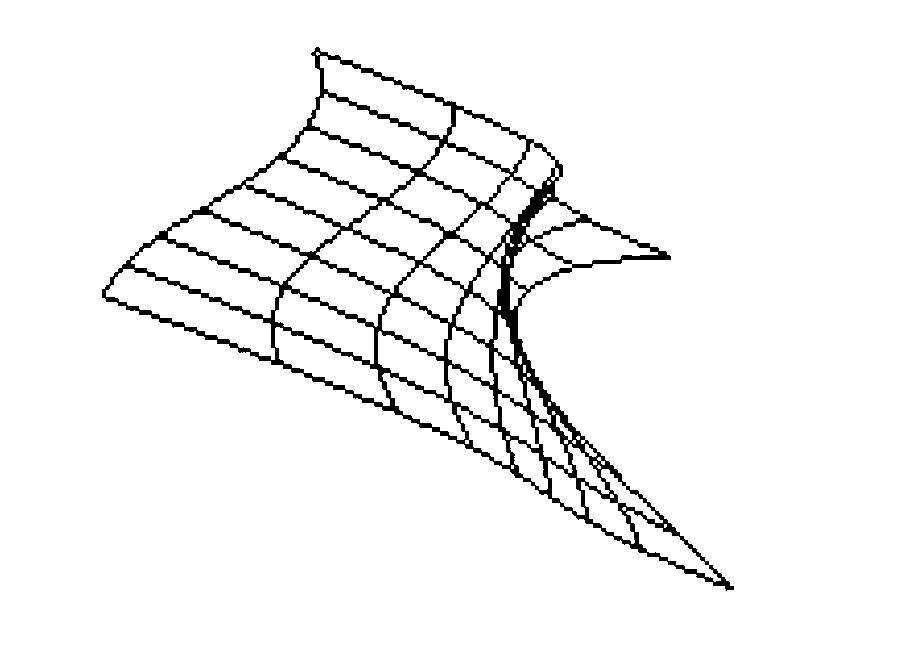
A parametric bivariate polynomial surface patch is used to represent a 3D curved surface. Points on the patch are defined by three bivariate polynomials, one each for x, y, z. The boundaries of the patch are parametric curves. Typically, a third degree bivariate polynomial is used which produces a bicubic patch. This is a much more efficient representation of a curved surface than a polygon mesh (fewer parametric patches needed for accuracy). This figure depicts a Bezier surface.
Quadric Surfaces
A quadric surface is implicitly defined by an equation f(x, y, z) = 0, where f is a quadric polynomial in x,y,z. Example quadrics are circles, spheres, ellipsoids, etc.
Polygon Meshes
A mesh is a set of vertices, edges, and polygons. Each edge in the mesh is shared by at most two polygons. An edge connects two vertices. A polygon is a closed sequence of edges.
The key issue with meshes is one of representation and the ensuing space/time tradeoffs.
An explicit mesh representation (Benefits ?/ Disadvantages?)
- requires that each polygon be specified by a list of vertices. Such a representation duplicates many vertices and does not identify shared vertices and edges. Rendering such a mesh would result in redrawing all shared edges. Thus, this representation is neither space nor time efficient.
A vertex pointer representation (Benefits ?/ Disadvantages?)
- requires that each polygon be specified as a list of pointers (indices) into a list of vertices. Each vertex is stored exactly once. The space overhead is the list of pointers maintained for each polygon. The representation identifies shared vertices but still does not identify shared edges so redrawing occurs. This representation is space efficient/time inefficient.
Example
VList = {V1, V2, V3, V4} where Vi = (xi, yi, zi) and Polygon1 = {1, 2, 4}, Polygon2 = {2, 3, 4}, ie. Two triangles are specified with a shared edge incident on vertices V2, V4.
End Example
An edge list representation (Benefits ?/ Disadvantages?)
- requires that each polygon be specified as a list of pointers (indices) into a list of edges. Each edge is stored exactly once. An edge is composed of its two vertices and the polygon to which it belongs. Each vertex is stored exactly once. The space overhead is the list of edges and the list of pointers for each polygon. To render an outlined mesh, it is necessary to render only the edge list. To render filled polygons is equally efficient. Shared edges are not redrawn. This representation is moderately space efficient and very time efficient.
Example
VList'={V1, V2, V3, V4} where Vi = (xi, yi, zi) and EList" ={E1, E2, E3, E4, E5} where E1 = {1', 2', P1, NULL}, E2 = {2', 4', P1, P2}, E3 = {1', 4', P1, NULL}, E4 = {2', 3', P2, NULL}, E5 = {3', 4', P2, NULL}, and P1 = {1", 2", 3"}, P2 = {2", 4", 5"}. Two triangles are specified with a shared edge E2 incident on vertices V2, V4.
End Example
Because of the complexity of representing meshes correctly, consistency checks are frequently carried out for a constructed mesh.
Issues of concern are : each edge is used, each vertex is incident on two edges, each polygon is closed, the mesh is connected, no holes in mesh, each polygon is planar, etc. The edge list representation is the most useful for such checks.
One neat application of polygonal meshes is the fractal generation of terrains such as mountain ranges. Troy Kozee's I.S. investigated this topic. The mesh is generated by starting with a unit square in the x-z plane. Recursive bilinear interpolation is used to construct an n x n grid of vertices within the unit square. The depth of the recursion defines the granularity of the mesh (the deeper the recursion the more polygonal patches generated). The y-coordinate of each vertex is then modulated using a fractal function to offset its value from the origin. Many kinds of functions can be applied to modulate y, but Troy used Fractal Brownian motion which produces very "noisy" results, ie. rugged, peaky mountains like the Rockies. An example screenshot of Troy's screen saver.
Parametric Cubic Curves
Parametric curves are represented by three equations
x = x(t), y = y(t), z = z(t)
which allows a curved surface to be approximated by a piecewise polynomial curve. The three equations above are cubic polynomials in the parameter t.
Cubic polynomials are used because this is the lowest order polynomial which allows non-planar curves to be expressed.
What is a non-planar curve? Why is a cubic polynomial the lowest order polynomial for non-planar curves?
- If we take the derivative of a quadratic polynomial at point
(x, y, z), what do we get?
- The slope of the tangent line at (x, y, z). So the "movement" along the curve at (x, y, z) is linear
- If we take the derivative of a cubic polynomial at point (x,
y, z), what do we get?
- A quadratic polynomial. So the "movement" along the curve at (x, y, z) is non-linear and may cross itself
Each cubic polynomial has the general form :
at3 + bt2 + ct + d
The four unknown coefficients (a, b, c, d) are solved for using four knowns (which might be the two endpoints of the curve and the derivatives of the endpoints or the unit tangent vectors at the endpoints).
The cubic polynomials required to specify a curved segment Q(t) are (EQS1):
x(t) = axt3 + bxt2 + cxt +dx
y(t) = ayt3 + byt2 + cyt +dy
z(t) = azt3 + bzt2 + czt +dz
Because we are dealing with finite curves, t is in the interval [0,1].
We can more compactly represent Q(t) as T*C where T is the row vector :
[ t3 t2 t 1]
and C is the 4 X 3 matrix :
| ax | ay | az |
| bx | by | bz |
| cx | cy | cz |
| dx | dy | dz |
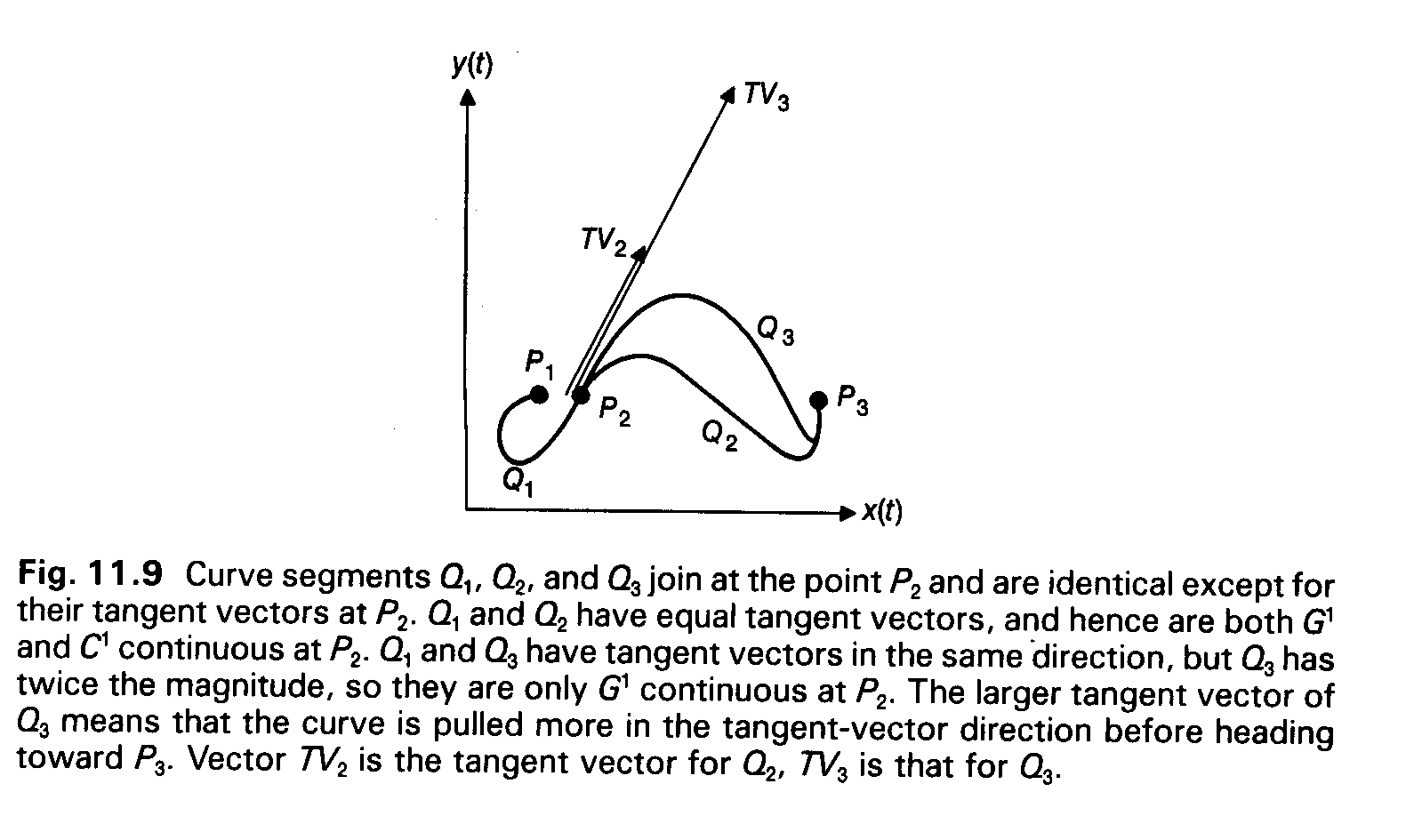
We can talk about the geometric continuity of two curves that meet at a join point. The continuity is expressed as a relation between the tangent vectors of the two curves. The tangent vector of a cubic curve is Q`(t) or T` * C =
- Go continuity exists if two curves join at a join point.
- G1 continuity exists if the direction of the two tangent vectors is equal.
- C1 continuity exists if the direction and magnitude of the two vectors is equal. Generally, C1 continuity implies G1 continuity.
- Cn continuity exists if the two vectors are equal through
the nth derivative. Refer to figures below.

[ 3t2 2t 1 0 ] * C
A curve Q(t) is defined by constraints on endpoints, tangent vectors, and continuity between curve segments.
The three types of cubic curves are
- hermite defined by two endpoints and two tangent vectors
- bezier defined by two endpoints and two other points that control the endpoint tangent vectors
- splines which are defined by 4 endpoints.
To see how the coefficients of EQS1 can depend on 4 unknowns rewrite
Q(t) = T*C as T*M*G where the coefficient matrix C = M*G.
M is a 4 x 4 basis matrix and G is a 4 element column vector of geometric constraints (endpoints or tangent vectors) called the geometry vector.
The elements of M and G are constants. Both M and G are
different for each type of curve. 
We now have to determine how to compute M for each type of curve.
Hermite Curves
The hermite curve is determined by constraints on the two given endpoints, P1, P4, and by constraints on the two tangent vectors, R1, R4, to the given endpoints.
To find the basis matrix, Mh, for a hermite curve
- construct four equations, one for each constraint, and solve for the four unknowns. The process is stated below for x(t) only, must be carried out for y(t) and z(t).
1. The parametric equation for x(t)
x(t) = axt3 + bxt2 + cxt + dx = T*Cx =
T*Mh*Gx
2. The geometry vector Gx captures contraints for the x coordinate of a point on the curve.
Remember that t is in the interval [0,1]. Substituting t = 0 into the parametric equations will give us point P1 on the curve. Substituting t = 1 into the equations will give us point P4 on the curve. Thus we constrain the curve to be finite and end on the given points.
T row vector
[ t3 t2 t 1]
Substitute t = 0 into the row vector for T to get, x(0) = P1x = | 0 0 0 1| *Mh*Gx. This is the constraint on x when t = 0.
Substitute t = 1 into the vector to get x(1) = P4x = |1 1 1 1|*Mh*Gx. This is the constraint on x when t = 1.
3. Determine the tangent vectors at P1 and P4 by calculating x`(t) =
[ 3t2 2t 1 0]
Substitute t = 0 into x`(t) to find x`(0) = R1x = |0 0 1 0|*Mh*Gx. This is the constraint on the tangent vector at P1 when t = 0.
Substitute t = 1 into x`(t) to find x`(1) = R4x = |3 2 1 0| *Mh*Gx. This is the constraint on the tangent vector at P4 when t = 1.
4. The four constraints for Gx =
| P1x = | 0 0 0 1 | ||
| P4x = | 1 1 1 1 | * Mh | * Gx |
| R1x = | 0 0 1 0 | ||
| R4x = | 3 2 1 0 |
5. Notice that the above equation is Gx = M*Mh*Gx where M is the expanded 4 X 4 matrix in step 4. The only way this equation can hold is if the basis matrix, Mh, is the inverse of M. We now have the method to solve for the basis matrix which is not done here, but is simply given.
Invert M to get Mh =
| 2 -2 1 1 |
| -3 3 -2 -1 |
| 0 0 1 0 |
| 1 0 0 0 |
If we wish to carry out the Hermite curve evaluation in matrix form then the structure is
| x(t) = | 2 -2 1 1 | P1x P1y P1z P1w | |||
| y(t) = | [ t3 t2 t 1] | * | -3 3 -2 -1 | * | P4x P4y P4z P4w |
| z(t) = | 0 0 1 0 | R1x R1y R1z R1w | |||
| w(t) = | 1 0 0 0 | R4x R4y R4z R4w |
T * Mh gives us the four Hermite blending functions, b0 = (2t3 -3t2 + 1), b1 = (-2t3 +3t2), b2 = (t3 -2t2 + t) and b3 = (t3 - t2)
and
| P1x P1y P1z P1w | ||
| [ b0 b1 b2 b3] | * | P4x P4y P4z P4w |
| R1x R1y R1z R1w | ||
| R4x R4y R4z R4w |
gives us Q(t) = b0*P1 + b1*P4 + b2*R1 + b3*R4
a point (x(t), y(t), z(t))on the curve, Q(t), is given by a weighted sum for each coordinate. For example
x(t) = b0*P1x + b1*P4x + b2*R1x + b3*R4x
y(t) = b0*P1y + b1*P4y + b2*R1y + b3*R4y
z(t) = b0*P1z + b1*P4z + b2*R1z + b3*R4z
w(t) is ignored.
Check out the code example (hermite.cpp).
Activity for hermite.cpp
- Reset the dimensions of the orthographic projection so the control points of hermite curve (end points and control points for tangents) will be visible in the view volume.
- Draw fat yellow points at the end points and control points.
- Draw red lines connecting end points to tangent vector control points.
- Does this clarify the relationship between control points
and the curve's structure?
Creating Joins for Hermite Curves
In order for two hermite curves to share an endpoint with G1 continuity then the following must hold for the geometry vectors of the two curves:
| C1 | C2 |
| P1 | P4 |
| P4 | P7 |
| R1 | kR4 |
| R4 | R7 |
where k > 0. So the tangent vectors at the shared endpoint, P4, must at least have equal directions. For C1 continuity to hold the tangent vectors at P4 must have equal magnitude and direction. (Command-option to emulate middle click on Mac track pad; brings up menu options on Example.
Bezier Curves
Bezier curves are specified using the two endpoints of the curve and two points not on the curve. The 4 points are referred to as control points. The control points define the convex hull of the curve where we might think of the hull as a bounding box that completely contains the curve. Note that all four control points do not have to lie on the convex hull boundary. Refer to figures below.
.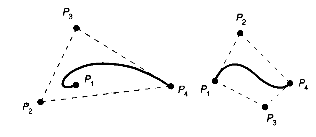
Let us refer to P1, P4 as the endpoints of the curve. P2, P3 are the control points which are used to define the tangent vectors at P1 and P4. The tangent vectors are determined by the vectors P2P1 and P4P3. These two vectors are related to the tangent vectors as follows :
R1 = Q`(0) = 3(P2-P1) and R4 = Q`(1) =3(P4-P3), EQs2.
The constant 3 is used to ensure that the curve has a constant velocity from P1 to P4 (refer to the 1st derivative of Q(t) to see why 3 is used).
The Bezier geometry vector Gb is merely :
| P1 |
| P2 |
| P3 |
| P4 |
The matrix Mhb that defines the relation between the Hermite geometry vector Gh and the Bezier geometry vector Gb (Gh = Mhb * Gb) is
| P1 | 1 | 0 | 0 | 0 | P1 | ||||
| Gh= | P4 | = | 0 | 0 | 0 | 1 | * | P2 | =Mhb*Gb |
| R1 | -3 | 3 | 0 | 0 | P3 | ||||
| R4 | 0 | 0 | -3 | 3 | P4 |
To find the Bezier basis matrix the following substitution is performed using the definition of a hermite curve:
Q(t) = T*Mh*Gh = T*Mh*(Mhb*Gb) [from above]
= T*(Mh*Mhb)*Gb = T*Mb*Gb. We know the basis matrix, Mh, for the hermite curve and Mhb is specified above so just carry out the multiplication to find Mb =
| -1 3 -3 1 |
| 3 -6 3 0 |
| -3 3 0 0 |
| 1 0 0 0 |
and the curve Q(t) = T*Mb*Gb is
Q(t) = (1-t)3P1 + 3t(1-t)2P2 + 3t2(1-t)P3 + t3P4
Note that the 4 weighting functions, bo = (1-t)3, b1 = 3t(1-t)2, b2 = 3t2(1-t) and b3 = t3 are formed by
[ t3 t2 t 1] *
and are referred to as the Bernstein Polynomials. Note that (1-t)3 = -t3 +3t2 -3t +1. This is what we get when we multiply T by column one of Mb above. The other weighting functions are produced similarly.
Creating Joins for Bezier Curves
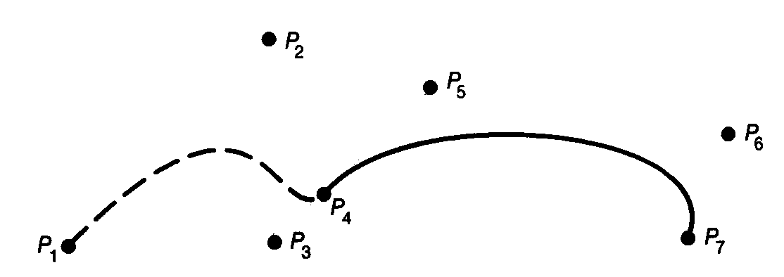
Assume we have two bezier curves. The first curve has endpoints P1, P4, and control points P2, P3. The second curve has endpoints P4, P7 and control points P5,P6. In order to create a join, with G1 continuity, for the two Bezier curves the following must be true : P4-P3 = k(P5-P4) with k > 0. This means the three points P3, P4, and P5 must be distinct and collinear. Refer to figure below.
Bezier Curves in OpenGL
OpenGL provides commands for creating Bezier curves directly. The process is fairly straightforward.
1. Define the geometry vector (specify control points) in a 4X3 array :
GLfloat cntrl[4][3] = {{-4.0,-4.0,0.0},{-2.0,4.0,0.0},
{2.0,-4.0,0.0},{4.0,4.0,0.0}};      //just an example
2. Define an evaluator which might be 2-D, 3-D, or 4-D. We will use a 3-D (3-D points on a curve) evaluator for this example. The evaluator can be in one parameter (for a curve) or 2 parameters (for a surface). The openGL command in one parameter is :
void glMap1[fd](GLenum target, TYPE u1, TYPE
u2, GLint stride, GLint order, const TYPE *points);
- target specifies what the control points represent (see table 12-1 in RedBook).
- u1 and u2 define the interval of values for the parameter t which might be [0.0,1.0] as in our discussion.
- stride defines the offset number to be used when accessing the geometry vector, in our case stride = 3.
- order is the degree (of the polynomial we are using) +1. Since the bezier is a cubic curve then the degree = 4. Note that order = # of control points.
- *points is the address of the first coordinate of the first control point. i.e. &cntrl[0][0].
So the call might look like : glMap1f(GL_MAP1_VERTEX_3,0.0,1.0,3,4,&cntrl[0][0]);
3. Enable the evaluator:
glEnable(GL_MAP1_VERTEX_3);
4. Perform the evaluation. Using a line strip, the
following command replaces the glVertx*() command:
void glEvalCoord1[fd](TYPE u); or
void glEvalCoord1[fd]v(TYPE *u);
where u is the value of the parameter (t) to be used in the evaluation. As an example:
glBegin(GL_LINE_STRIP); //or GL_POINT
for(int i = 0; i < 30; i++)
glEvalCoord1f(i/30.0);
glEnd();
An example program can be found in bezcurve.c. Look at source for command ordering.
If you wish to define evenly spaced values along the curve (as in the above example) it is much easier and more efficient to replace steps 3). and 4). above with :
3a. Enable the evaluator:
glEnable(GL_MAP1_VERTEX_3);
glMapGrid1(30, 0.0,1.0);
where void glMapGrid1(GLint n, TYPE u1,
TYPE u2) defines a map that goes from u1 to u2 in n evenly
spaced steps.
4a. Perform the evaluation. The for loop is now replaced as :
glEvalMesh1(GL_LINE, 0, 1);
where void glEvalMesh1(GLenum mode, GLint
p1, GLint p2) evaluates the mesh from p1 to p2. p1 >=u1, p2
<= u2. The mode may be GL_LINE/GL_POINT.
Activity for bezier.cpp
- Change the example program to use 3a) and 4a) steps described immediately above.
An Example for joined Bezier.
Parametric Bicubic Surfaces
The general form for a parametric curve is Q(t) = T*M*G where the geometry vector, G, is a constant. A surface can be defined by allowing the geometry vector to vary in a second parameter.
| G1(t) | |
| Q(s ,t) = S*M* | G2(t) |
| G3(t) | |
| G4(t) |
For a fixed ti, Q(s, ti) is a curve because G(ti) is a constant. Allowing t to vary over the interval of [0,1] creates a family of curves which define a surface. If the Gi(t) are cubics then the surface is a parametric bicubic surface.
We will not discuss hermite surfaces since openGL does not support any direct way of implementing them. An iterative solution (an extension to the iterative solution for the hermite curve) is not very efficient. Creation of the geometry vectors is a real pain (8 tangent vectors and 4 partial derivatives with respect to t and s).
Instead we will look at Bezier surfaces which are directly supported in openGL.
Bezier Surfaces (Parametric bicubic surface)
The bezier formulation is :
x(s,t) = S*Mb*Gx*Mb^*T^ where ^ represents transpose and Mb is the bezier basis matrix.
y(s,t) = S*Mb*Gy*Mb^*T^
z(s,t) = S*Mb*Gz*Mb^*T^
The bezier geometry vector contains 16 control points.
Bezier Surfaces in OpenGL
OpenGL provides commands for creating Bezier surfaces directly.
1. Define the geometry vector (specify control points) in a 4X4X3 array :
GLfloat cntrl[4][4][3];
Use the following grid to visualize the ordering of control points in the geometry vector:
| a41 | a42 | a43 | a44 |
| a31 | a32 | a33 | a34 |
| a21 | a22 | a23 | a24 |
| a11 | a12 | a13 | a14 |
control[4][4][3] =
{{{a11},{a12},{a13},{a14}},
{{a21},{a22},{a23},{a24}},
{{a31},{a32},{a33},{a34}},
{{a41},{a42},}a43},{a44}}};
2. Define a 2 parameter evaluator which might be 2-D, 3-D, or 4-D. We will use a 3-D (3-D points on a surface) evaluator for this example. The openGL command in two parameters is :
void glMap2[fd](GLenum target, TYPE u1, TYPE
u2, GLint ustride, GLint uorder,
TYPE
v1, TYPE v2, GLint vstride, GLint vorder, const TYPE *points);
- target specifies what the control points represent (as in table 12-1 but use MAP2).
- u1, u2 and v1, v2 define the interval of values for the parameters s and t respectively which might be [0.0,1.0] as in our discussion.
- ustride, vstride defines the offset number to be used when accessing the geometry vector.
- uorder, vorder is the degree (of the polynomial we are using) +1. Since the bezier is a cubic curve the degree = 4.
- *points is the address of the first coordinate of the first control point. i.e. &cntrl[0][0][0].
So the call might look like :
glMap2f(GL_MAP2_VERTEX_3, 0.0, 1.0, 3, 4,
0.0, 1.0, 12, 4, &cntrl[0][0]);
Note the vstride (above = 12) which is moving across all columns in a row (4*3).
3. Enable the evaluator:
glEnable(GL_MAP2_VERTEX_3);
4. Perform the evaluation. The following command replaces the glVertex*() command:
void glEvalCoord2[fd](TYPE u,TYPE v);
or
void glEvalCoord2[fd]v(TYPE *u, TYPE *v);
where u,v is the value of the parameter (s/t) to be used in the evaluation. As an example:
for(int i = 0; i <= 8; i++)
glBegin(GL_LINE_STRIP);//GL_POINT
for(int j = 0; j <=
30; j++)
glEvalCoord2f(j/30.0,
i/8.0);
glEnd();
glBegin(GL_LINE_STRIP);//GL_POINT
for(int j = 0; j <=
30; j++)
glEvalCoord2f(i/8.0,
j/30.0);
glEnd();
If you wish to define evenly spaced values along the surface (as in the above example) it is much easier and more efficient to replace steps 3). and 4). above with :
3a. Enable the evaluator:
glEnable(GL_MAP2_VERTEX_3);
glMapGrid2(8, 0.0,1.0,30,0.0,1.0);
where void glMapGrid(GLint n1, TYPE u1,
TYPE u2, GLint n2,TYPE v1, TYPE v2) defines a map that goes from
u1 to u2 in n1 evenly spaced steps and from v1 to v2 in n2 evenly
spaced steps.
4a. Perform the evaluation. The nested for loop is now replaced as :
glEvalMesh2(GL_LINE, 0, 1,0,1);
where void glEvalMesh2(GLenum mode, GLint
p1, GLint p2, GLint p2, GLint p4) evaluates the mesh from p1 to
p2 and from p3 to p4. p1 >=u1, p2 <= u2 and p3>=v1, p4<=
v2. The mode may be GL_POINT/GL_LINE/GL_FILL.
Activity - complete the bezier mesh started in bezmesh.c. The example shows a lighted bezier surface with normals automatically generated. Control points are also drawn.
Demo example Bezier surface.
Uniform Nonrational B-Splines (curves)
B-splines are made up of curve segments where each curve segment depends on only four control points. Adjacent curve segments share control points. This is how continuity between segments is maintained. A curve segment may not necessarily pass through its control points.
A cubic b-spline approximates a series of m+1 control points:
P0, P1, ..., Pm, m >= 3,
with a curve made up of m-2 cubic polynomial curve segments; Q3, Q4,...Qm.
The cubic polynomial is parameterized in t (as previous discussions) but the domain of t
is modified to be t = t+k.
This allows the domain of t to be sequential for each curve segment. Thus the parameter t for Qi
is defined on the interval ti<=t<=ti+1, for 3<=i<=m.
In the case where m=3
there is a single curve, Q3, defined on the interval, t3<=t<=t4, by 4 control points, P0,..,P3.
For m > 3 or (for each i >= 4) there is a join point or knot between curve segment Qi and
Qi+1 at the parameter value ti. See figure. The initial value of ti
(t3) and the final value of ti (tm+1) are also called knots. Thus a b-spline curve contains a total of m-1 knots.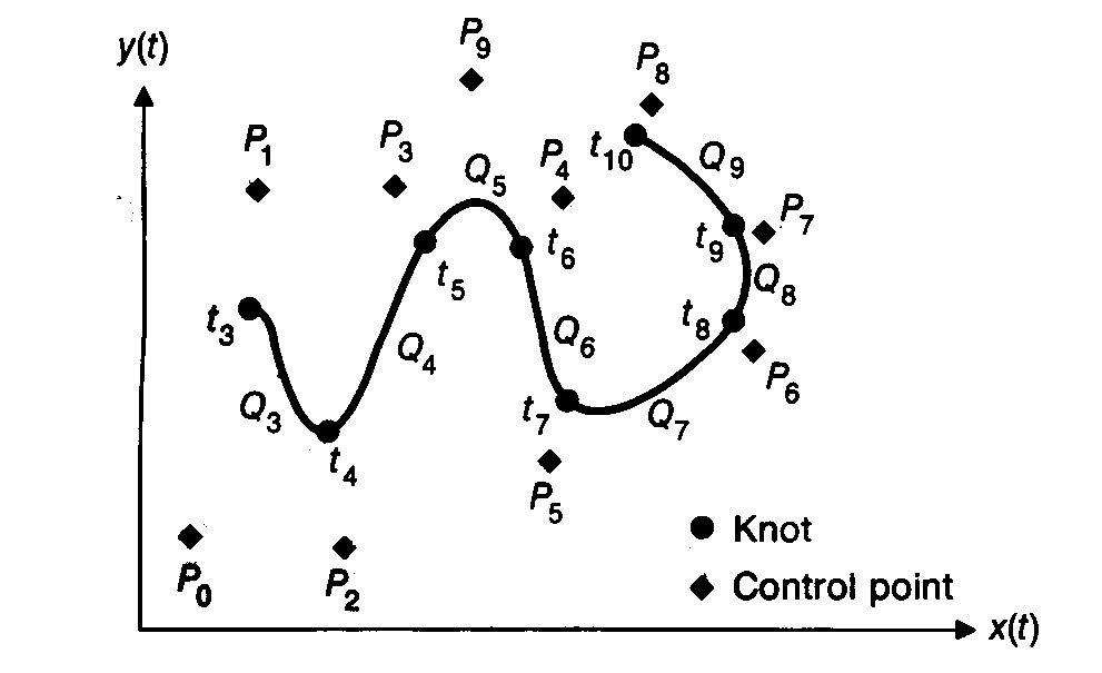
The term uniform means that the knots are spaced at equal intervals of the parameter t.
Assume that t3 = 0 and that ti+1 - ti = 1.
B-splines may be non-rational or rational (where x(t), y(t), and z(t) are a ratio of two cubic polynomials).
B stands for "basis" because the splines are represented as a weighted sum of polynomial basis functions (as we did for hermite/bezier curves).
The Geometry Vector for B-splines
Each of the m-2 curve segments in a spline is defined by four of the m+1 control points. Curve segment Qi is defined by the controls, Pi-3, Pi-2, Pi-1, Pi. In general the geometry vector
Gsi =
| Pi-3 |
| Pi-2 |
| Pi-1 |
| Pi |
As depicted in the drawing, the first curve segment Q3 is controlled by points P0,P1,P2,P3 over the parameter range t3 = 0 to t4 = 1. The two knots are t3 and t4. Each curve segment Qi is contained within the convex hull of its 4 control points. The second curve segment Q4 is controlled by points P1, P2, P3, P4 over the parameter range t4 = 1, t5 = 2. Additional segments are defined in a similar manner.
It should be clear that many of the control points (except for those at the beginning/end of the sequence) control four curve segments. Thus moving one control point can move the four curve segments it controls.
Ti is defined as the row vector [(t-ti)3, (t-ti)2, (t-ti), 1].
The curve segment Qi is defined as Ti * Ms * Gsi for ti <= t <= ti+1.
The entire curve is generated by applying the above equation for 3 <= i <= m.
The basis matrix Ms is derived in[BART87] =
| -1 , 3 , -3 , 1 | |
| 1/6* | 3 , -6 , 3 , 0 |
| -3 , 0 , 3 , 0 | |
| 1 , 4 , 1 , 0 |
Adjacent curve segments in a b-spline exhibit C0, C1, and C2 continuity where they join (magnitude and direction of tangent vectors at a knot are equal through the 2nd derivative). This tends to make b-spline curves smoother than either hermite or bezier curves.
Nonuniform Nonrational B-splines
Splines in this class allow a nonuniform spacing between knots. The advantage of nonuniform spacing is the ability to easily add an additional knot and control point so the resulting curve is reshaped.
In order to specify a nonuniform spacing for knots, a knot sequence must be supplied.
- The knot sequence values must be non-decreasing.
- The sequence must contain knots t3, .., tm+4 (there are four more knots than control points).
- For a b-spline made up of a single segment, Q3, with four control points, an 8 knot sequence is provided over the parameter interval [0,1].
The only restriction on the knot sequence is that it is non-decreasing, thus multiple knots may have the same parameter value. This occurrence is called a multiple knot and the number of knots with the same parameter value is called the multiplicity of the knot. In the knot sequence, [0,0,0,0,1,1,1,1], the knot value = 0/1 both have multiplicity 4.
When a multiple knot occurs (ti = ti+1), the curve segment Qi reduces to a single point. This allows nonuniform nonrational b-splines to be more flexible than the uniform case. Use figure 11.27 as an example to see how knot multiplicity affects the resulting curve.
a). If each ti of Qi is unique then multiplicity =
1 and all curve segments have C0,C1,C2 continuity at the knots.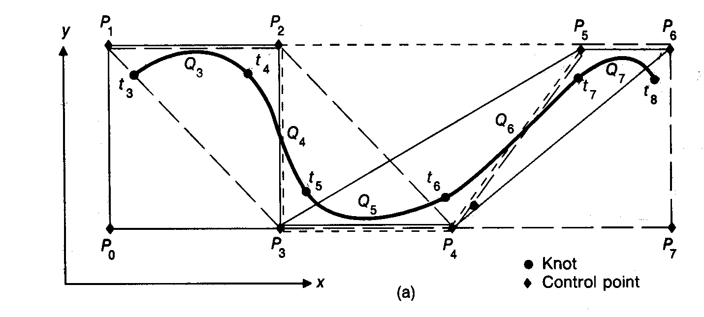
b). If ti = ti+1 then multiplicity = 2. The knot
ti lies in the convex hull defined by Pi-3,Pi-2,Pi-1 and the knot ti+1
lies in the hull defined by Pi-2, Pi-1, Pi. This means the two knots
lie on the line segment defined by Pi-2, Pi-1 : the shared boundary of
their respective convex hulls. The curve segment Qi thus degrades to
the shared knot point. The join now has C1 continuity.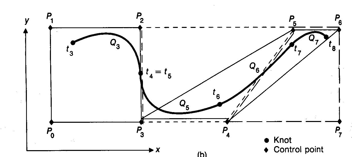
c). If ti = ti+1 = ti+2 then multiplicity = 3.
This means the three knots lie on control point Pi-1. Curve segments Qi
and Qi+1 degenerate to points. The join now has C0 continuity.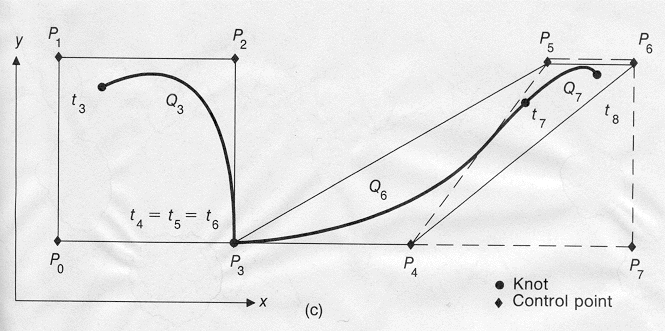
d). If ti = ti+1 = ti+2 = ti+3 then multiplicity =
4. The four knots cause a discontinuity because the curve segments, Qi
and Qi+4 contain no common control points. The curve doesn't even have
G0 continuity.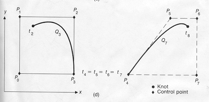
As an aside, the knot sequence, [0,0,0,0,1,1,1,1], causes the b-spline to degrade to a bezier curve for each remaining unjoined curve segment (see above figure).
Demo nonuniform spline.
Nonuniform Rational Cubic Polynomial Curve Segments (NURBS)
General rational cubic curve segments are defined by:
x(t) = X(t)/W(t), y(t) = Y(t)/W(t), z(t) = Z(t)/W(t) where X,Y,Z, and W are all cubic polynomials with control points defined as homogeneous coordinates. So any non-rational curve can be transformed to a rational one by merely adding W(t) = 1 as a fourth element.
Thus Q(t) = [X(t), Y(t), Z(t), W(t)].
The curve Q(t) can be a hermite, bezier or other type. When the curve is a b-spline it is referred to as a NURBS.
Rational curves (splines) are useful because they are invariant under rotation, scaling, translation, and perspective transformation of the control points. Non-rational curves are invariant only under scaling, rotation, and translation.
What does this mean?
For rational curves, the perspective transformation needs only be applied to the control points.
Rational splines can also be used to specify any conic section (using quadratic polynomials, not cubic).
B-Spline Surfaces
B-splines patches are represented as :
x(s,t) = S*Ms*Gsx*Ms^*T^ where ^ is used to signify transpose.
y(s,t) = S*Ms*Gsy*Ms^*T^
z(s,t) = S*Ms*Gsx*Ms^*T^
where C2 continuity across boundaries is automatic with b-splines.
SKIP:Why is an 8 knot sequence required for NURBS? (same issue for either curves or surfaces - discussion deals with curves)
In General: Blending Functions
All of the curves and surfaces we have discussed so far have associated blending functions. The blending functions are defined to be T*M where M is the basis matrix for the type of curve/surface of interest. Remember that each of the curves are defined as a parametric polynomial Q(t) = T*M*G where G is the geometry vector for the curve. The blending functions are just weighted sums which are then applied to the geometry matrix. The weighted sums are in the form of a cubic polynomial in the parameter t. As an example lets look at x(t) = T*M*G.
x(t) =( t^3m11 +t^2m21 +tm31+m41)g1x + (t^3m12+t^2m22+tm32+m42)g2x +(t^3m13+t^2m23+tm33+m43)g3x+(t^3m14+t^2m24+tm34+t44)g4x
Thus, for hermite/bezier curves there are 4 blending functions defined (one each as applied to the gix components above).
Blending Functions for NURBs
As a reminder, the b-spline (NURB) formulation for curve segment Qi = Ti*Mb*Gsi for ti<=t<=ti+1.
The b-spline blending functions are given by the product, Ti*Mb. There are 4 blending functions, each applied to its respective control point in the geometry vector :
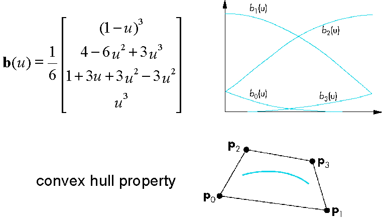
A complexity arises with NURBS because they are specified with nonuniform intervals between knot values. Thus there is no single set of blending functions as there are for the other types of curves. Instead the four blending functions are defined recursively in terms of lower-order blending functions.
The eight knots are required in order to compute the four recursive blending functions. This computation is quite costly and a strong argument for restricting knot intervals to 0 or 1. In such a case the table depicted in the drawing can be stored as a small set of precomputed matrices.
So, an 8-knot sequence is minimally required and any curve defined with m control points must have an m+4 knot sequence.
OpenGL NURBS
NURBS are supported via the Glu library package.
If you want to set up lighting for a nurbs surface
use glEnable(GL_AUTO_NORMAL) to generate surface normals
automatically (or calculate your own). Use glEnable(GL_NORMALIZE)
if you are using scaling to transform your curve or surface. This
command will renormalize the surface normals so lighting calculations
will be correct.
Managing NURBS in OpenGL (curves or surfaces)
1. Create a NURBS object using:
GLUnurbsObj* gluNewNurbsRenderer(void);
returns a pointer to the nurbs object which is used in subsequent
commands.
2. Destroy the NURBS object using :
void gluDeleteNurbsRenderer(GLUnurbsObj
*nobj);
If you have a chance to look at the GLU documentation you will see that a large number of callback functions can be defined for NURBS management. Minimally it seems like a good idea to provide an error callback in case an error condition occurs (there are 37 errors specific to NURBS). The syntax to do so follows:
//To handle GLU version differences
#ifndef CALLBACK
#define CALLBACK
#endif
//CallBack function
void CALLBACK nurbsError(GLenum errorCode)
{
const GLubyte *estring;
estring = gluErrorString(errorCode);
fprintf (stderr, "Nurbs Error:
%s\n",estring);
exit (0); }
//register CallBack function, placed after
//command to create the NURB
gluNurbsCallback(theNurb, GLU_ERROR,
(GLvoid (*)()) nurbsError);
NOTE: Not working in my SDK, working in newer version of SDK.
4. Specify the control points as (x,y,z) or (x,y,z,w) in an array of floats. For a curve with m-2 curve segments provide m+1 control points. For a surface provide a grid of control points. For a surface made up of single curve segments you will have to specify (4x4) 16 control points. For more complicated surfaces made up of multiple curve segments, extend the grid dimensions.
5. Specify the knot sequence (ti) as an array of floats. For a curve with m-2 curve segments provide m+4 knots. For a surface made up of single curve segments provide an 8-knot sequence for each of the s,t parameters. The same knot sequence can be used for both. For a surface made up of multiple curve segments the knot sequence must be extended in size.
Managing NURBS Curves
1. To render a NURBS curve use a begin/end pair as in :
void gluBeginCurve(GLUnurbObj *nobj);
void gluEndCurve(GLUnurbObj *nobj);
2. To display the curve use:
void gluNurbsCurve(GLUnurbObj *nobj, GLint
nknots, GLfloat *knot, GLint stride, GLfloat *cntrpts, GLint order,
GLenum type);
- nobj = NURBS object
- nknots = knot sequence size
- knot = array of knots
- stride = size of a column in control pointer array
- cntrpts = control points array
- order = degree of polynomial + 1
- type = GL_MAP1_VERTEX_3/_4
Example
//11 control points and 15 knots to define 8
curve //segments for the b-spline
gluBeginCurve(theNurb);
glColor3f(1.0, 0.0, 0.0);
gluNurbsCurve(theNurb, 15, knots, 3,
&ctlpoints[0][0], 4, GL_MAP1_VERTEX_3);
gluEndCurve(theNurb);
End Example
Managing NURBS Surfaces
1. Define the properties you want associated with the NURBS using:
void gluNurbsProperty(GLUnurbsObj * nobj,
GLenum property, GLfloat value);
Properties and associated values are:
GLU_DISPLAY_MODE : GLU_FILL (default),
GLU_OUTLINE_POLYGON, GLU_ OUTLINE_PATCH.
GLU_NURBS_MODE : GLU_NURBS_RENDERED
(default=>renders surface),
GLU_NURBS_TESSELLATOR (allows access to
tessellated data)
.
GLU_CULLING: GL_TRUE (tessellation not
performed if surface not in view vol.), GL_FALSE (default).
A NURBS surface is rendered as a set of primitives (line segments or polygons). This is done by sampling the curves at different values for the s,t parameters to construct the primitives. It is possible to set the sampling property you wish to use for the surface rendering via :
GLU_SAMPLING_METHOD : just use the default which
is GLU_PATH_LENGTH (default). Other possible values are
specified on page 519.
The other available properties are linked to the sampling method used (investigate on your own).
Example
/*displaymode is a GLfloat : used to
toggle between Fill and Outline modes based on user input*/
gluNurbsProperty(theNurb,
GLU_DISPLAY_MODE, displaymode);
/*using the default sampling method of
path length, setting the maximum edge length of the tesselated polygons
in pixels.*/
gluNurbsProperty(theNurb,
GLU_SAMPLING_TOLERANCE, 25.0);
End Example
2. To get the properties of a NURBS use :
void gluGetNurbsProperty(GLUnurbsObj *nobj,
GLenum property, GLfloat *value);
3. To render a NURBS surface use a begin/end pair as in :
void gluBeginSurface(GLUnurbObj *nobj);
void gluEndSurface(GLUnurbObj *nobj);
4. To display the surface use:
void gluNurbsSurface(GLUnurbObj *nobj, GLint
sknots, GLfloat *sknot, GLint tknots, GLfloat *tknot,
GLint s_stride, GLint t_stride, GLfloat *cntrpts, GLint
sorder, GLint torder, GLenum type);
where type is either GL_MAP2_VERTEX_3/_4.
Other parameters as for a curve.
Example
/*An 8 knot sequence for
paramters s,t, a 4x4 array of control points which defines only a
single curve segment for all curves that specify the surface*/
gluNurbsProperty(theNurb,
GLU_DISPLAY_MODE, displaymode);
gluBeginSurface(theNurb);
gluNurbsSurface(theNurb, 8, knots, 8,
knots, 4 * 3, 3, &ctlpoints[0][0][0], 4, 4, GL_MAP2_VERTEX_3);
gluEndSurface(theNurb);
End Example
Refer to the text example in surface.c.
GLU Quadric surfaces
The quadric surfaces are defined as analytical functions. Glu supports spheres, cylinders and disks.
1. To create/delete a quadric use:
GLUquadricObj* gluNewQuadric(void);
void gluDeleteQuadric(GLUquadricObj* qobj);
2. To register an error callback (refer to NURBs error callback example) use:
void gluQuadricCallback(GLUquadricObj* qobj,
GLenum which, void (*fn)());
The only legal value for which is GL_ERROR.
3. To define rendering style use:
void gluQuadricDrawStyle(GLUquadricObj*
qobj,GLenum drawStyle);
where drawStyle may be GLU_POINT, GLU_LINE,
GLU_FILL, GLU_SILHOUETTE.
4. To generate normals use:
void gluQuadricNormals(GLUquadricObj*
qobj,GLenum normals);
where normals may be GLU_NONE, GLU_FLAT, GLU_SMOOTH.
5. To generate texture coordinates use:
void gluQuadricTexture(GLUquadricObj* qobj,
GLboolean texcoords);
where texcoords is either GL_TRUE or
GL_FALSE.
6. The quadric primitives are
a. void gluSphere(GLUquadricObj*
qobj,GLdouble radius, GLint slices, GLint stacks);
b. void gluCylinder(GLUquadricObj*
qobj,GLdouble baseRadius,Gldouble topRadius, GLdouble height, GLint
slices, GLint stacks);
c. void gluDisk(GLUquadricObj*
qobj,GLdouble innerRadius, GLdouble outerRadius, GLint slices, GLint
stacks);
d. void gluPartialDisk(GLUquadricObj*
qobj,GLdouble innerRadius, GLdouble outerRadius, GLint slices,GLint
rings, GLdouble startAngle, GLdouble sweepAngle);
Refer to the text example in quadric.c.

