Lab 1 - 10pts
For this lab, you will be learning to use DataSpell from JetBrains, an IDE for data science with intelligent Jupyter notebook and Python script.
This is an extraordinarily useful tool for all kinds of engineering analysis and design. In the notebook we can quickly and interactively test solutions out, and in a Python script we can create a complete solution as a stand alone program. One advantage of the Jupyter notebook, is that it is a webapp and thus platform independent.
Installing DataSpell:
-
Before we start you need to have Python 3.10 or higher. MacOS includes Python; on Windows systems, Python must be installed. In either system, start by checking if you have Python installed by typing in a command window:
which Python
If you have Python, check to see if it is version 3.10 or higher by typing in a command window:
Python –version
or Python –VIf you do not have Python 3.10 or higher, please install it from <https://ww.python.org/downloads/
- You need to have Miniconda Python installed (this is an open-source package management system). For this, Google “download miniconda” a process which most likely will take you to this webpage. Select the appropriate installer, 64 bit for Windows and for MacOS, select pkg M1 or Intel (pkg, not bash), depending on what processor you have (check it via System Preferences – Processor). Install Miniconda.
- Next you install DataSpell. You will need an account with JetBrains, which is free for education; it is the same company that offers CLion we use for C++ programming.
- If you already have the JetBrains Toolbox installed, simply click the Install button next to DataSpell tool. Otherwise, Google “download DataSpell”, a process which most likely will take you to this webpage. Select MacOS or Windows download based on your laptop and proceed to install.
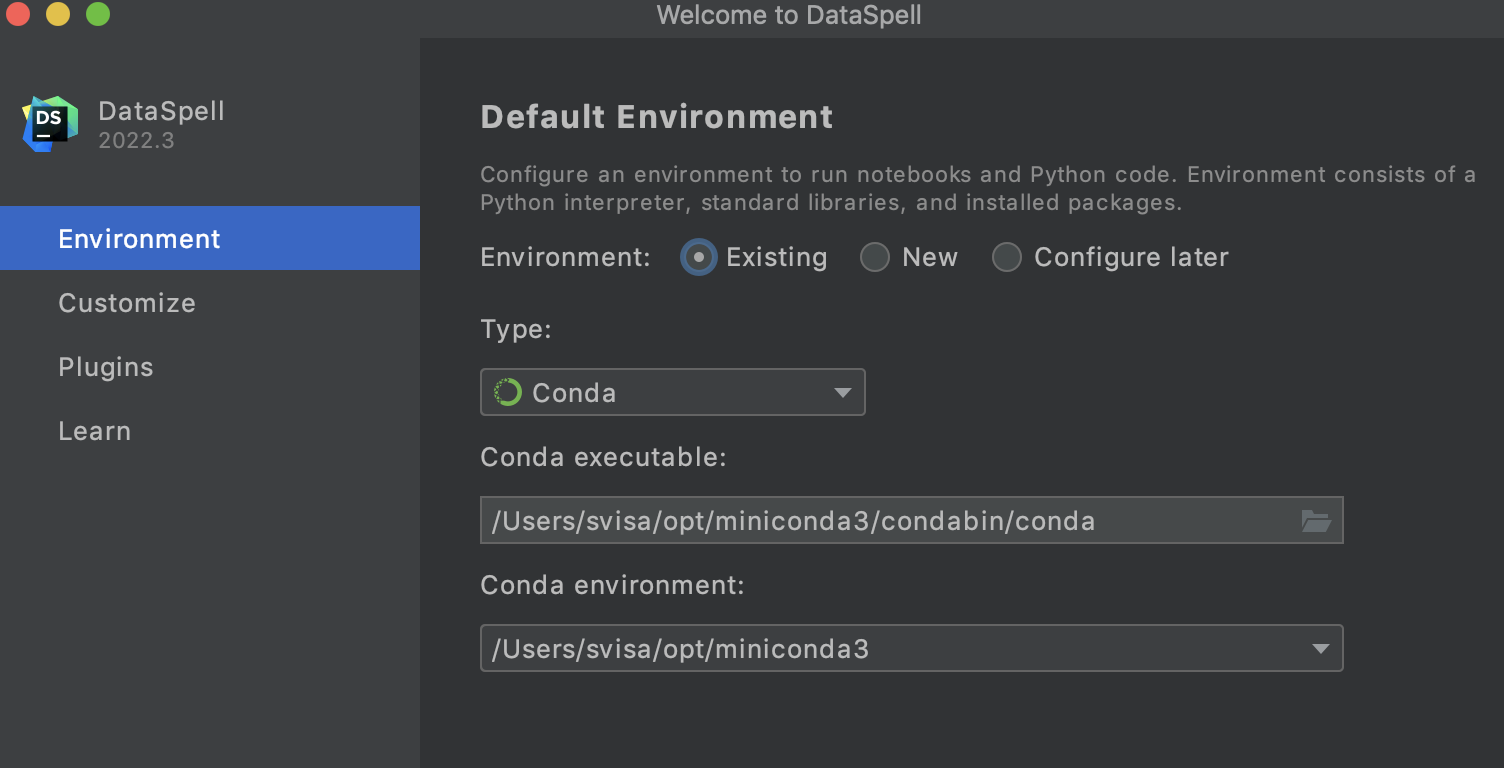
- Launch DataSpell. It will ask you to select the Default Python Environment, which by default is Conda, so you should leave it as shown in the picture below.
Now you are done with the installation part, great!
Complete the tasks described below. At the end of the lab, you will
(1) (6pts) upload a Word document with answers to the seven problems from below; the work for these problems will be in the notebook which also gets uploaded.
(2) (4pts) upload the zipped up project folder Lab1 containing your code work in Lab1_Notebook.ipynb and Lab1_File.py.
Part A) For this part you will be entering your commands in the Lab1_Notebook.ipynb
- Start DataSpell
- In the top tab “Files”, select “New Workspace Directory” and name it Lab1.
- Right-click Lab1 and select “New” than select “Jupyter Notebook” and name it Lab1_Notebook.
- Right-click Lab1 and select “New” than select “Python File” and name it Lab1_File.
- Select the
Lab1_Notebook.ipynband in its first cell let’s import three libraries, math, numpy, and matplotlib; in Pyhton comments start with#
# for python documentation see <https://docs.python.org/3/
import math
# importing library - see more info at numpy.org
import numpy as np
# importing library - see more info at matplotlib.org
import matplotlib.pyplot as plt
# if it says you do not have it, right-click the red lightbulb anf select "Install it"
Let’s create a list using the commands in green. Type the command in green, run the cell, and observe the output shown in red. To tun a cell, click the green “Run Cell” triangle; alternatively, to run an active cell you may click Shift+Enter keys, or you may right-click in a cell and select “Run Cell”.
a = [1, 2, 4, 5]
print(a)
a
    [1, 2, 4, 5]
    [1, 2, 4, 5]
In another cell, let’s verify that a is a list.
# a is a list
type(a)
    list
Let’s create a row vector from the list a.
# creating a row vector
vector1 = np.array(a)
print(vector1)
vector1
  [1 2 4 5]

 1
 2
 4
 5
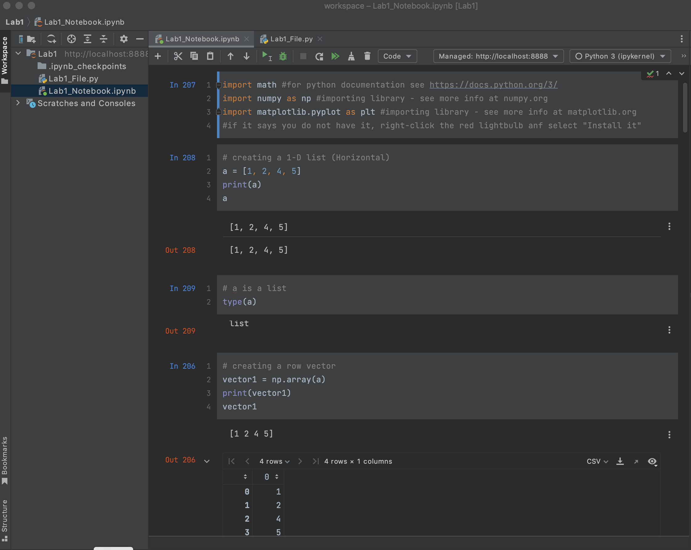
To run all cells, click the “Run All” button shown as two-overlayed green triangles. You should see a screen similar to the one below.
In another cell, let’s verify that vector1 is a vector.
# vector1 is a list
type(vector1)
    numpy.ndarray
Vectors
If you aren’t comfortable with matrices, you might want to refer to the References section on the course webpage. Now using the transpose comand from the numpy library we create a column vector as shown below. Remember, a transpose is obtained by switching rows and columns in a matrix - so the transpose of a row vector is a column vector.
# creating a column vector
b = [[3], [-1], [-2], [3]]
vector2 = np.array(b)
print(vector2)
vector2
[[ 3]
[-1]
[-2]
[ 3]]

3
-1
-2
3
Now using a command from the numpy library we can multiply the vectors:
# multiply the vectors as dot-product
np.matmul(vector1, vector2)
8
1) Verify, by hand on the Word documeny, the calculation of vector1 * vector2.
Matrices
A matrix can be entered as a list of lists and then transfomed into a 2D array.
# creating a 2 x 2 matrix
A = [[1, -2], [1, 2]]
A = np.array(A)
print(A)
np.shape(A)

     1    -2
     1     2
(2, 2)
The identity matrix can be formed with the function identity(n), where n is the size of the desired matrix.
I = np.identity(2)
I

     1     0
     0     1
We can now do mathematic manipulations of these matrices, including finding the inverse of the matrix A. Recall that \(A*A^{-1} = I\) (where \(A^{-1}\) is the inverse of A).
np.matmul(A,I)

     1    -2
     1     2

np.matmul(I,A)

     1    -2
     1     2

# compute the inverse of matrix A
A_prime = np.linalg.inv(A)
print(A_prime)
np.matmul(A, A_prime)

    0.5000    0.5000
-0.2500    0.2500
1     0
0     1
2) Verify, by hand, the calculation of A*A_prime.
Matrix Applications
Matrices can be used to solve multiple simultaneous equations. For example, consider the problem of solving 3 simultaneous equations:
This can be written in a matrix form as

where
3)Verify the preceding statement (i.e., show thatAx=b represents the set of equations). For instance, first equation is obtained as 1x1 + 2x2 + 3*x3 = 0.
One can solve these equations by various substitution methods or can use matrices.

To do this using Python notebook, do the following:
A = np.array( [[1, 2, 3], [1, -1, 2], [3, 1, -1]] )
b = np.array( [[0], [-2], [5]] )
x = np.matmul( np.linalg.inv(A) , b)
print(x)

     1
     1
    -1
which is the correct solution. [You may verify, by replacing in the three equations x1 by 1, x2 by 1, and x3 by -1, and see that the equations hold true.]
4) What are x1, x2, x3, and x4 for the following set of equations? Use your Python notebook to get the solution.In word doc write thee solution only.
Static equilibrium problem: A picture hangs on the wall from two strings as shown. The picture has a mass of two kilograms. We can sum the forces in each direction, where T1 and T2 are the tensions in the strings.
5) Find T1 and T2, using Python notebook and write your solution in the Word doc.
(Note: you’ll have to move the “mg” term to the right hand side of the second equation). It is the product of mass (2kg) and g=9.80665 Newtons/kg. You can use Python notebook to find the sine and cosine, but first you must convert the angle to radians:
np.cos(30*math.pi / 180)

    0.8660

np.sin(30*math.pi / 180)

    0.5000
or you could use the fact that
or, with Python (using the Square RooT function - sqrt()).
math.sqrt(3)/2

    0.8660
Plotting functions
Python’s matplotlib can be useful as a tool for plotting functions. For example, lets plot a sinusoidal function.
First, generate a time vector that will be used for plotting.
t = np.arange(0, 10, 0.1)
This generates a vector t that goes from 0 to 10 with an incremental value of 0.1. In other words t=[0 0.1 0.2 ... 9.9 10.0].
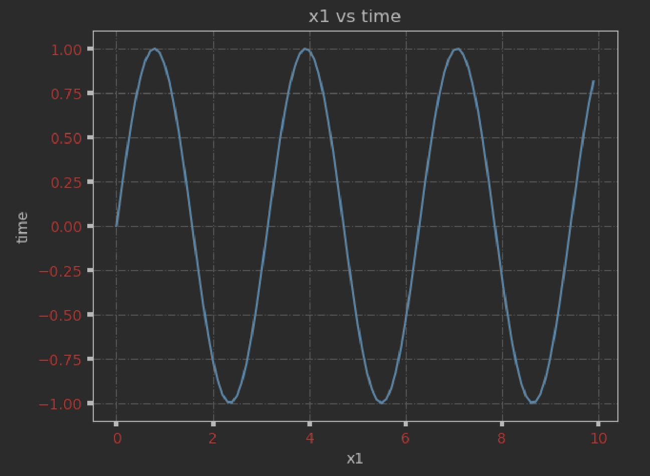
Now lets create another vector, x1, that is the sine of t, with a frequency of 2 radians per second. Then we’ll plot it.
x1 = np.sin(2 * t)
Create just a figure and only one subplot
fig, ax = plt.subplots()
ax.plot(t, x1)
ax.set_title("x1 vs time")
ax.set_xlabel('x1')
ax.set_ylabel('time')
ax.grid(True, linestyle='-.')
ax.tick_params(labelcolor='r', labelsize='medium', width=3)
plt.show()
The resulting figure should look like the one shown below.
Now let’s create and plot some more functions. At this point it is useful to point out that the up and down arrow buttons before the run button help you move cells up or down. Also, if you want to insert a new cell in-between two cells, hover your mouse over the top of the second cell and select “Add code cell”.
x1 = np.cos(t);
x2 = np.cos(3*t)/9;
x3 = np.cos(5*t)/25;
x4 = np.cos(7*t)/49;
x5 = np.cos(9*t)/81;
plt.plot(t, x1, color='blue')
plt.plot(t, x2, '--', color='green')
plt.plot(t, x3)
plt.plot(t, x4)
plt.plot(t, x5,)
plt.legend( ['x1', 'x2', 'x3', 'x4' , 'x5'] )
plt.xlabel('Time (t)')
plt.ylabel('x1-x5 functions')
plt.title('Five functions vs time')
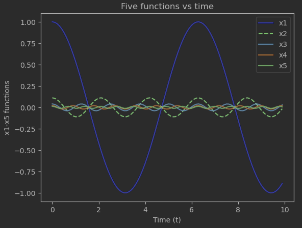
While there is no obvious relationship between these functions, one can be found. In a new cell, plot the sum of the 5 vectors; it should represent a triangle wave. This is a demonstration that any function can be made up of sine waves.
6) Copy-paste in the Word document the clearly labeled graph of the resulting approximation to a triangle wave. To copy-paste your plot from the DataSpell notebook, in MacOS press Cmd+Shift+4 keys and select the figure by dragging the mouse over the region you want to select. When you release the keys, the picture will be saved as png on your desktop. In Windows, press Ctrl+ PrtScn keys; the entire screen changes to gray including the open menu. Select Mode, select the kind of snip you want, and then select the area of the screen capture that you want to capture.
Subarrays
In Python, it is also possible to work with just parts of arrays. For example, if we want to plot just the first 50 points of the array x1, we can use the colon operator, “:”, to take indices 1 through 50 (1:50).
t = np.arange(0, 10, 0.1)
x1 = np.sin(2 * t)
plt.plot(t[1:50], x1[1:50])
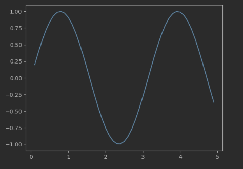
7) In an new cell use the colon operator to plot the function defined by x1 and t for one period starting near the zero crossing at t = 1.5 seconds. Copy-paste the resulting graph in the Word document.
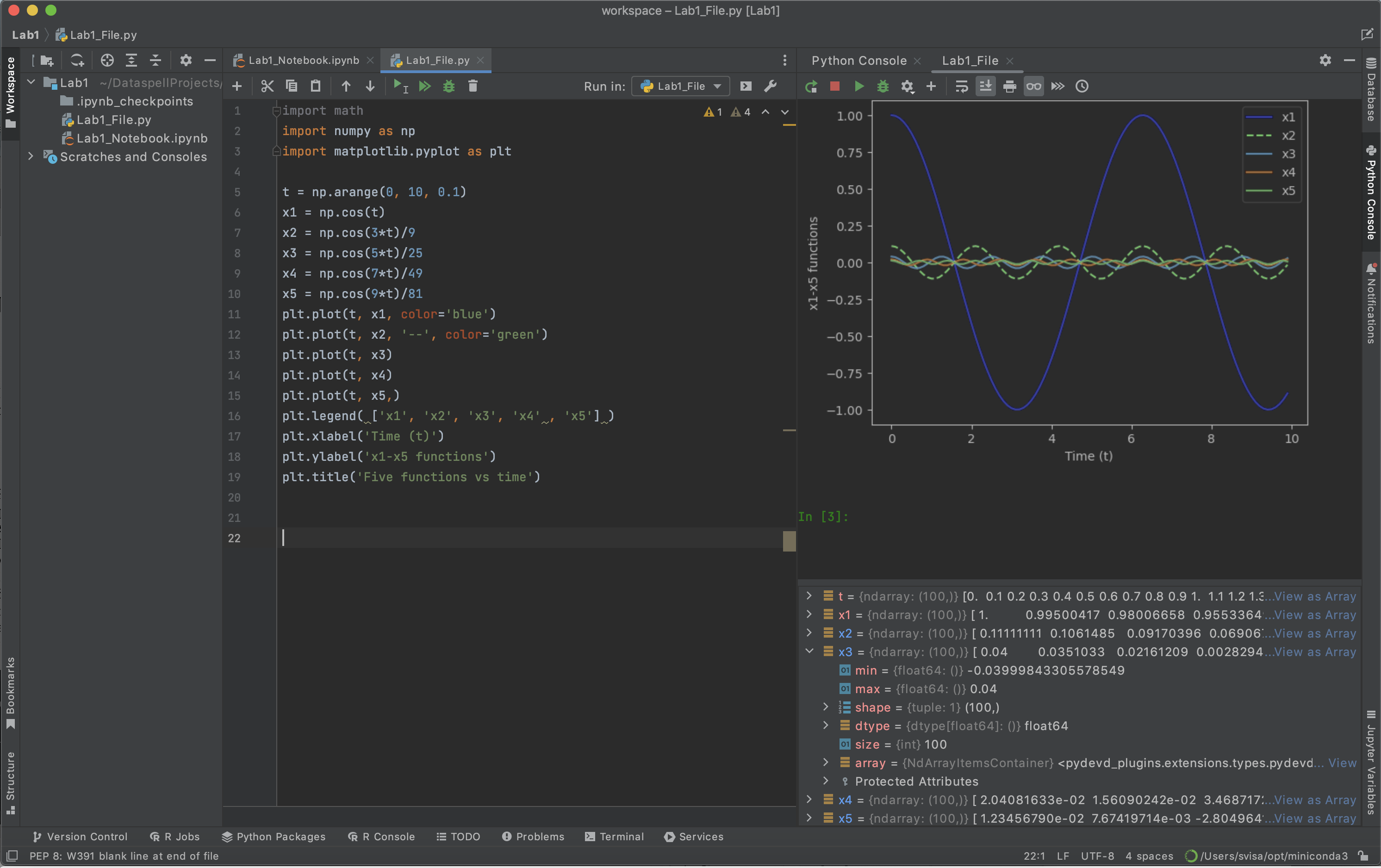
Part B) For this part you will be entering your commands in the Lab1_File.py
Copy-paste the following code in your Lab1_File.py file and click the green run button.
import math
import numpy as np
import matplotlib.pyplot as plt

x1 = np.cos(t)
x2 = np.cos(3*t)/9
x3 = np.cos(5*t)/25
x4 = np.cos(7*t)/49
x5 = np.cos(9*t)/81
plt.plot(t, x1, color='blue')
plt.plot(t, x2, '--', color='green')
plt.plot(t, x3)
plt.plot(t, x4)
plt.plot(t, x5,)
plt.legend( ['x1', 'x2', 'x3', 'x4' , 'x5'] )
plt.xlabel('Time (t)')
plt.ylabel('x1-x5 functions')
plt.title('Five functions vs time')
plt.show()
You should see something similar to the screen below. This shows that in DataSpell IDE we can also create complete Python programs in addition to using the Python notebook as a developping tool.